Linear Regression with Gradient Descent and Python
Gradient Descent is the key optimization method used in machine learning. Understanding how gradient descent works without using API helps to gain a deep understanding of machine learning. This article will demonstrates how you can solve linear regression problem using gradient descent method.
Our test data (x,y) is shown below. It is a simple linear function 2*x+3 with some random noise
import numpy as np
import matplotlib.pyplot as plt

x = np.linspace(0,10,20)
y = 2*x+3+2*np.random.rand(len(x))

plt.scatter(x,y)
plt.show()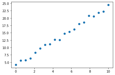
We use a model given by yhat = w*x +b. The loss function is a Mean Square Error (MSE) given by the mean sum of (yhat-y)**2. We compute the gradients of the loss function for w and b, and then update the w and b for each iteration. We output the final w, b, as well as the loss in each iteration.
def gradientDescent(x, y, theta, learn_rate, N, n_iter):
    loss_i = np.zeros(n_iter)
    for i in range(n_iter):
        w = theta[0]
        b = theta[1]
        yhat = w*x+b
        loss = np.sum((yhat-y)** 2)/(2*N)
        loss_i[i] = loss
        print("i:%d, loss: %f" % (i, loss))

        gradient_w = np.dot(x,(yhat-y))/N
        gradient_b = np.sum((yhat-y))/N
        w = w - learn_rate*gradient_w
        b = b - learn_rate*gradient_b
        theta = [w,b]
    return theta,loss_i
We set the hyperparametrs and run the gradient descent to determine the best w and b
n_iter = 100
learn_rate = 0.05
theta = np.zeros(2)
N = len(x)

theta,loss = gradientDescent(x, y, theta, learn_rate, N, n_iter)
print(theta)
After the iteration, we plot of the best fit line overlay to the raw data as shown below
import matplotlib.pyplot as plt

plt.plot(x,y,'or')
plt.plot(x,theta[0]*x+theta[1],'b')
plt.show()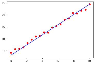
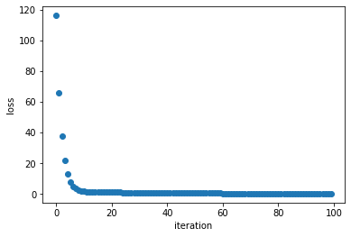
We also plot the loss as a function of iteration. The loss reduces with time indicating the model is learning to fit to the data points
import matplotlib.pyplot as plt

epoch = range(len(loss))
plt.plot(epoch,loss,'o')
plt.xlabel('iteration')
plt.ylabel('loss')
plt.show()