Comparison of LSTM, GRU and RNN on Time Series Forecasting with Pytorch
In this article, we will compare the performance of LSTM, GRU and vanilla RNN on time series forecasting using Pytorch Deep Learning platform.
Given a time series data for airline passengers as shown below. There is a obvious growth trend and a seasonal cyclic pattern in the data.
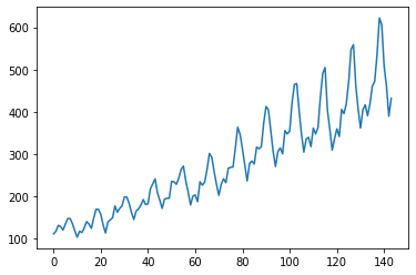
We can construct LSTM, GRU or RNN model using Pytorch to predict the time time series.
The LSTM model code
class LSTM(nn.Module):

    def __init__(self, num_classes, input_size, hidden_size, num_layers):
        super(LSTM, self).__init__()

        self.num_classes = num_classes
        self.num_layers = num_layers
        self.input_size = input_size
        self.hidden_size = hidden_size
        self.seq_length = seq_length

        self.lstm = nn.LSTM(input_size=input_size, hidden_size=hidden_size,
                            num_layers=num_layers, batch_first=True)

        self.fc = nn.Linear(hidden_size, num_classes)

    def forward(self, x):
        h_0 = torch.zeros(self.num_layers, x.size(0), self.hidden_size)
        c_0 = torch.zeros(self.num_layers, x.size(0), self.hidden_size)

        # Propagate input through LSTM
        _, (h_out, _) = self.lstm(x, (h_0, c_0))
        h_out = h_out.view(-1, self.hidden_size)
        out = self.fc(h_out)

        return out
The RNN model can be shown below:
class GRU(nn.Module):

    def __init__(self, num_classes, input_size, hidden_size, num_layers):
        super(GRU, self).__init__()

        self.num_classes = num_classes
        self.num_layers = num_layers
        self.input_size = input_size
        self.hidden_size = hidden_size
        self.seq_length = seq_length

        self.gru = nn.GRU(input_size=input_size, hidden_size=hidden_size,
                            num_layers=num_layers, batch_first=True)

        self.fc = nn.Linear(hidden_size, num_classes)

    def forward(self, x):
        h_0 = torch.zeros(self.num_layers, x.size(0), self.hidden_size)

        # Propagate input through LSTM
        _, h_out = self.gru(x, h_0)
        h_out = h_out.view(-1, self.hidden_size)
        out = self.fc(h_out)

        return out
Finally the RNN model is shown below:
class RNN(nn.Module):

    def __init__(self, num_classes, input_size, hidden_size, num_layers):
        super(RNN, self).__init__()

        self.num_classes = num_classes
        self.num_layers = num_layers
        self.input_size = input_size
        self.hidden_size = hidden_size
        self.seq_length = seq_length

        self.rnn = nn.RNN(input_size=input_size, hidden_size=hidden_size,
                            num_layers=num_layers, batch_first=True)

        self.fc = nn.Linear(hidden_size, num_classes)

    def forward(self, x):
        h_0 = torch.zeros(self.num_layers, x.size(0), self.hidden_size)

        # Propagate input through LSTM
        _, h_out = self.rnn(x, h_0)
        h_out = h_out.view(-1, self.hidden_size)
        out = self.fc(h_out)

        return out
To form the data, we can define a sliding window to scan the training data
def sliding_window(data, seq_length):
    x = []
    y = []

    for i in range(len(data)-seq_length-1):
        _x = data[i:(i+seq_length)]
        _y = data[i+seq_length]
        x.append(_x)
        y.append(_y)

    return np.array(x),np.array(y)
To test the model, we can split the time series data into training and. testing set
train_size = int(len(y) * 0.67)
test_size = int(len(y)) - train_size
dataX = torch.Tensor(np.array(x))
dataY = torch.Tensor(np.array(y))
trainX = torch.Tensor(np.array(x[0:train_size]))
trainY = torch.Tensor(np.array(y[0:train_size]))
testX = torch.Tensor(np.array(x[train_size:len(x)]))
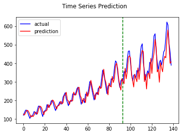
testY = torch.Tensor(np.array(y[train_size:len(y)]))The result for the time series forecasting is shown below
LSTM
GRU

RNN
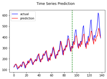
The comparison of the results show that LSTM modeling is sightly than GRU and RNN>