Time Series Forecasting using Tensorflow Keras
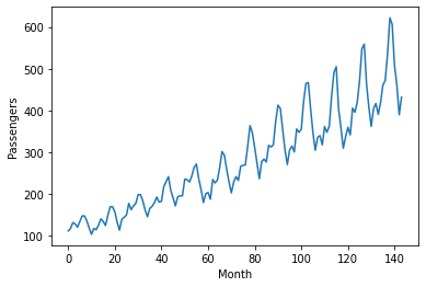
Recurrent Neural Network (RNN) model has been very useful to predict time series data.. Training on Tensorflow Keras is a great platform to implement RNN as the learning curve is less steep as compared to other platforms eg Training on Pytorch. In this article, we will demonstrate how to apply the LSTM model with Tensorflow Keras to model time series. We will use Airline passengers data as example..
The LSTM model for the stock price is shown below
model = Sequential()
model.add(LSTM(hidden_size, activation='tanh',input_shape=(timesteps,feature)))
model.add(Dense(1,activation='linear'))

model.compile(loss='mse', optimizer='adam')
history = model.fit(trainX, trainY, epochs=1000)
To form the data, we can define a sliding window to scan the training data
def sliding_window(data, seq_length):
    x = []
    y = []

    for i in range(len(data)-seq_length-1):
        _x = data[i:(i+seq_length)]
        _y = data[i+seq_length]
        x.append(_x)
        y.append(_y)

    return np.array(x),np.array(y)
To test the model, we can split the time series data into training and. testing set
sc = MinMaxScaler()
dataset = sc.fit_transform(dataset)

timesteps = 4
X,y = sliding_window(dataset, timesteps)

train_size = int(len(y) * 0.67)
test_size = int(len(y)) - train_size

X_train = X[0:train_size]
y_train = y[0:train_size]

X_test = X[train_size:len(x)]
y_test = y[train_size:len(y)]

feature = 1
hidden_size = 5

# inputs: A 3D tensor with shape [batch, timesteps, feature].
X_train = np.reshape(X_train, (X_train.shape[0], timesteps, input_size))
X_test = np.reshape(X_test, (X_test.shape[0], timesteps, 1, input_size))
We can plot the actual and predicted stock prices using scikit learn and matplotlib libraries
loss = history.history['loss']
epoch = range(len(loss))

import matplotlib.pyplot as plt

plt.plot(epoch,loss)
plt.xlabel('Epoch')
plt.ylabel('Loss]')
plt.show()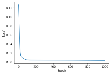
yhat = model(X)

yhat = sc.inverse_transform(yhat)
y_ = sc.inverse_transform(y)

plt.axvline(x=train_size, c='g', linestyle='--')

plt.plot(y_,'b',label='actual')
plt.plot(yhat,'r',label='prediction')
plt.xlabel('Month')
plt.ylabel('Airline Passengers')
plt.legend()
plt.show()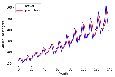
The result shows that LSTM model is extremely good in predicting the time series